Can you detail the Monte Carlo method in reinforcement learning, breaking down each step of the algorithm and providing a comprehensive explanation?🔗

Monte Carlo Methods:🔗

Monte Carlo methods in reinforcement learning are a way to estimate value functions and derive optimal policies from them. They are based on averaging sample returns. Since MC methods require actual returns for learning, they can only be applied to episodic tasks.

MC Algorithm:🔗

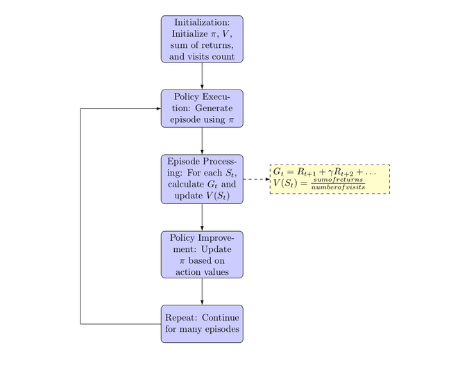
1. Initialization:

   • Initialize an arbitrary policy $\pi$.
   • Initialize value function $V$ for all states, typically to zeros.
   • Create empty lists or counters to keep track of the sum of returns and the number of visits for each state.

2. Policy Execution:

   • Using the policy $\pi$, generate an episode: $S_0, A_0, R_1, S_1, A_1, R_2, \dots, S_T$, where $S_T$ is a terminal state.

3. Episode Processing:

   • For each state $S_t$ appearing in the episode:
     • Calculate the return $G_t$ as the sum of rewards from time $t$ onwards. Typically, it's discounted:
       $$G_t = R_{t+1} + \gamma R_{t+2} + \gamma^2 R_{t+3} + \dots$$
     • Append $G_t$ to the list of returns for state $S_t$.
     • Update the value of $S_t$ as the average of its returns:
       $$V(S_t) = \frac{\text{sum of returns for } S_t}{\text{number of times } S_t \text{ has been visited}}$$

4. Policy Improvement (for MC Control):

   • If the goal is not just to evaluate a policy but also to improve it (MC Control), then:
     • Update the policy at each state based on the action that maximizes expected returns (e.g., using the Q-values).
     • Continue generating episodes and updating the policy until it stabilizes.

5. Repeat:

   • Repeat steps 2-4 for a large number of episodes to ensure accurate value estimates.

Explanation:🔗

MC methods are fundamentally about learning from episodes of experience.

• Sampling: Instead of knowing the complete dynamics of the environment (like in Dynamic Programming methods), MC methods rely on episodes sampled from the environment to gather information.

• Averaging Returns: The core idea behind MC is straightforward: to find the value of a state, simply average the total returns observed after visiting that state over many episodes.

• Epsilon-Greedy Exploration: To ensure adequate exploration of all state-action pairs, an ε-greedy policy (or other exploration strategies) might be employed, especially in MC control where the goal is to find the optimal policy.

• No Bootstrapping: Unlike Temporal Difference methods, MC does not bootstrap. This means it waits until the final outcome (end of the episode) to calculate the value of a state based on actual returns rather than estimating it based on other estimated values.

Example:🔗

Imagine teaching an agent to play a simple card game like Blackjack.

• You start with a random policy, like "always stick if I have 20 or 21, otherwise hit."
• The agent plays many games (episodes) of Blackjack against the dealer.
• After each game, the agent goes back through the states it was in during the game and calculates the total return from each state (sum of rewards until the end of the game).
• The agent then updates the estimated value of each state based on these returns.
• If doing MC control, the agent would also adjust its policy over time, deciding whether to stick or hit based on which action has historically given better returns from each state.

Over time, after many games, the value estimates will converge to the true expected returns, and the policy (if being optimized) will approach the optimal strategy for playing Blackjack.

---

Key equations for the Monte Carlo (MC) methods and explain each:

1. MC Prediction (State Values):🔗

For a given policy $\pi$, the objective is to estimate the state-value function $V^\pi(s)$.

Key Equation:

Here, the return $G_t$ is the total discounted reward from time $t$ onwards:

Explanation: The value of a state $S_t$ is updated by averaging over all the returns that have been observed after visiting that state across different episodes.

2. MC Prediction (Action Values):🔗

For a given policy $\pi$, the objective is to estimate the action-value function $Q^\pi(s, a)$.

Key Equation:

With the return $G_t$ defined as before.

Explanation: Similar to state values, but here the value is associated with taking a specific action $A_t$ in a specific state $S_t$. The update is an average of all returns observed after taking action $A_t$ in state $S_t$ across different episodes.

3. MC Control: GLIE (Greedy in the Limit with Infinite Exploration):🔗

The goal is to improve the policy over time to converge to the optimal policy $\pi^*$.

Key Equations:

Policy Improvement:

Where $\arg\max_a$ chooses the action $a$ that maximizes $Q(s, a)$ for state $s$.

Explanation: After estimating $Q(s, a)$ values using MC prediction, the policy is improved by choosing the action that maximizes expected return in each state. Exploration is ensured using strategies like ε-greedy, with $\epsilon$ decreasing over time to ensure the "Greedy in the Limit" property.

4. MC Control: Constant-α:🔗

This is a variant of MC Control that uses a constant step size $\alpha$ for updates.

Key Equation:

Explanation: Instead of averaging all returns for a state-action pair, this method takes a weighted average of the old value and the new return. The weight is given by $\alpha$, the learning rate. This approach can be more suitable for non-stationary environments where recent returns might be more relevant than older ones.

In all these methods, the core idea is to use actual returns observed from episodes to update value estimates, either for evaluation (MC Prediction) or for improving the policy (MC Control).